Scalable Bayesian Optimization of Black-Box Functions

These are the slides I presented at my university a while ago on my research regarding scalable BO. In this presentation I provided a decision-theoretic roots of Expected Improvement (EI) acquisition function.

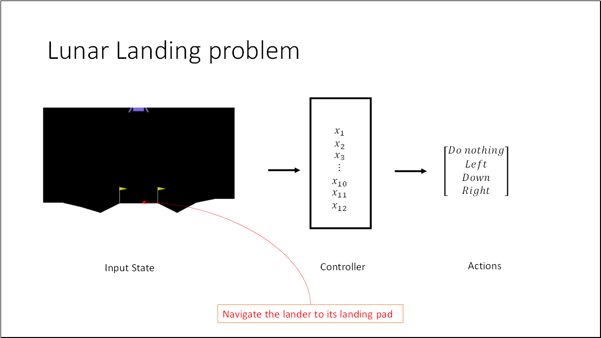
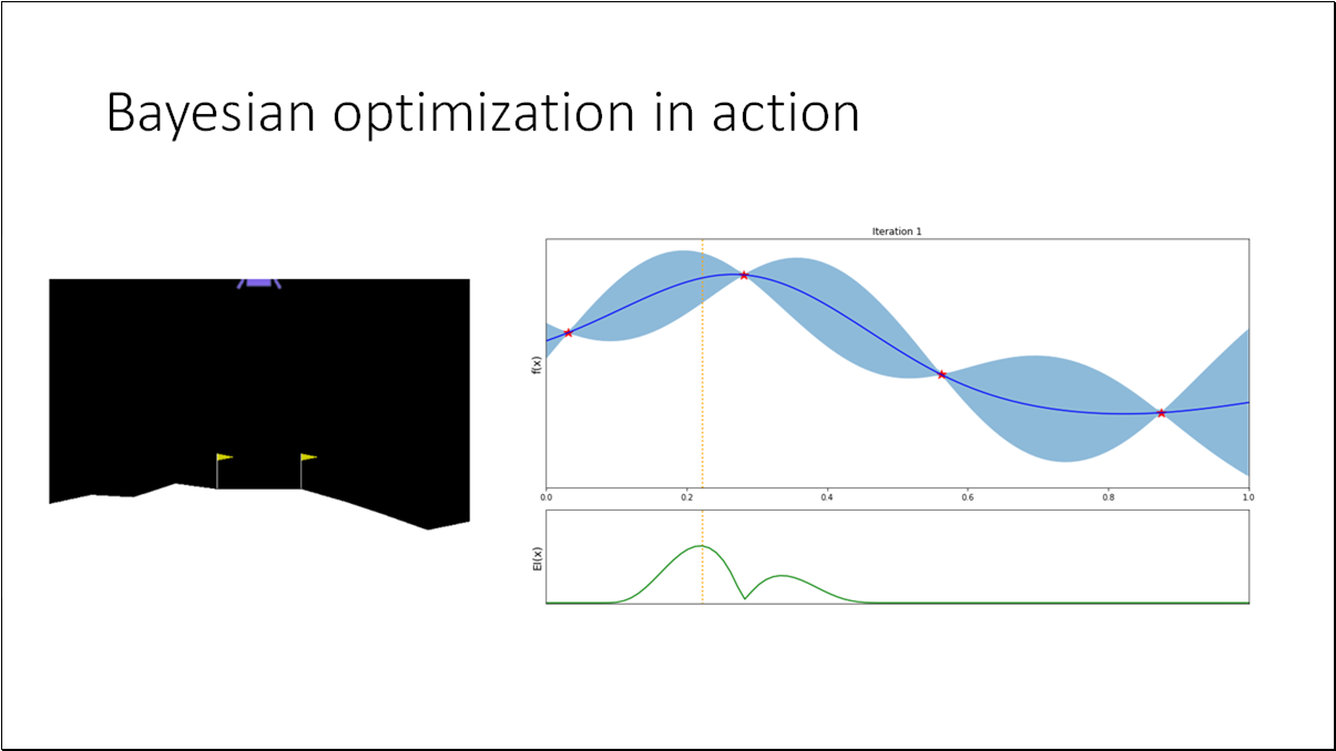
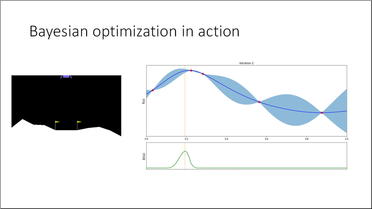
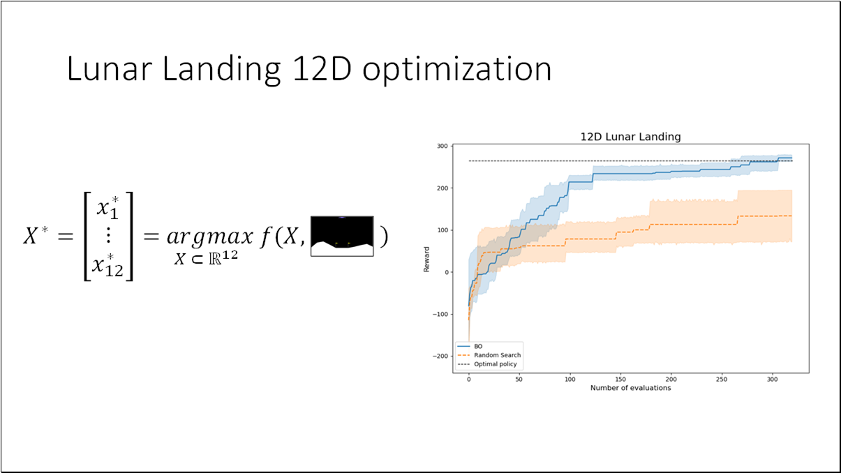
We will utilize the Lunar Landing problem from OpenAI Gym. The objective is to guide the lander to its landing pad. This presents an optimal control challenge, where we need to determine 12 parameters in the controller. Given an input state, these parameters will dictate one of four discrete actions.

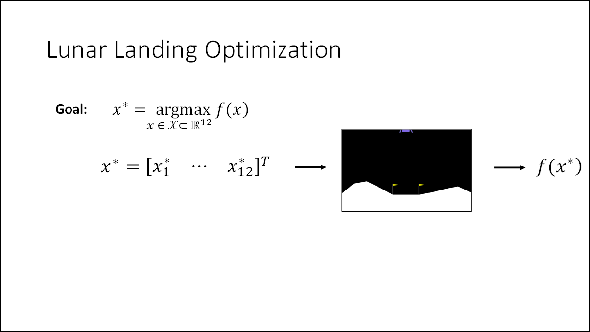
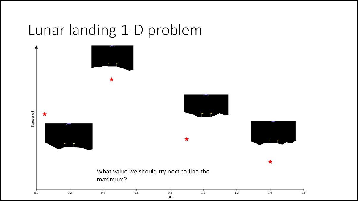
The lunar landing problem is a black box optimization problem. The goal is to find the parameters from our search space that maximize the objective function. The objective function $f$ is termed a black-box function if it meets one or more of the following criteria.

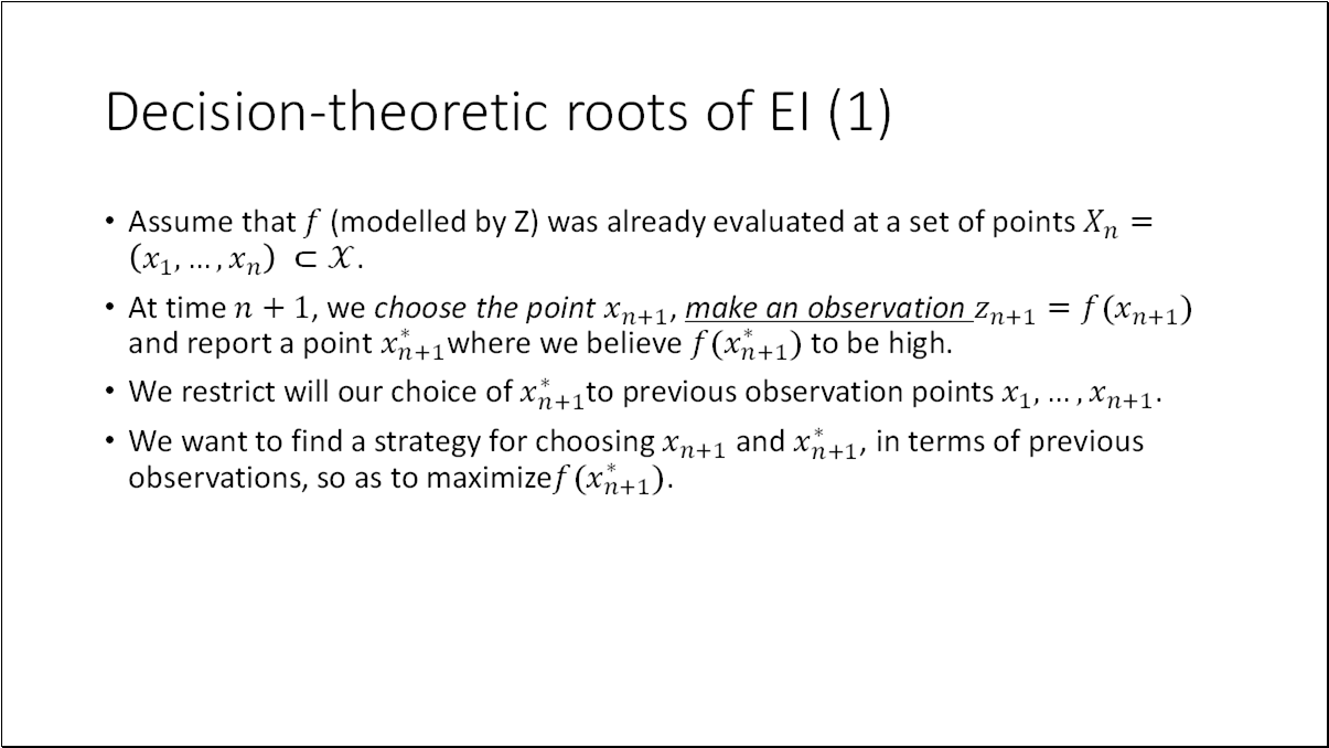
We can only obtain value points for the black-box function $f$ by querying its function values at arbitrary points $x \in \mathcal{X}$.

$x$ is an element of the index set $\mathcal{X}$. This index set is a proper subset of the set $\mathbb{R}^d$. The set $\mathbb{R}^d$ encompasses the entire space of tuples of size $d$.

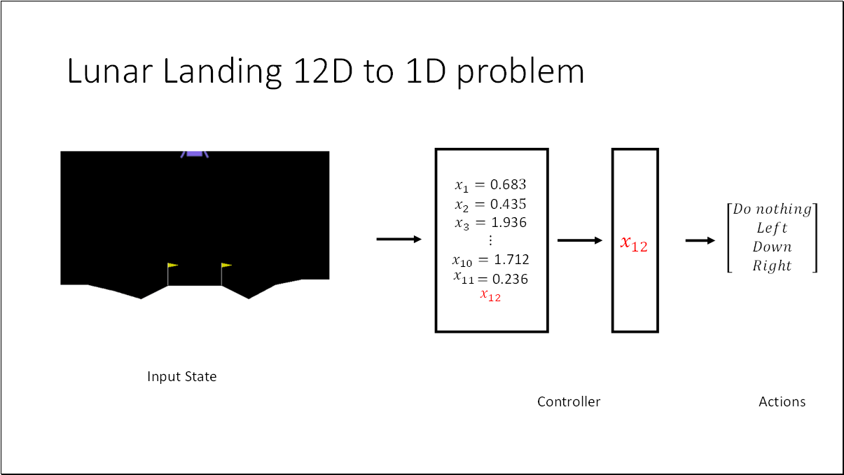
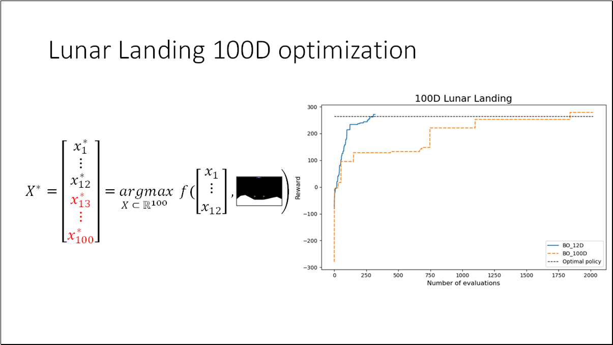
For the purpose of better visualization, we can convert the (12D) problem to a (1D) problem by fixing all the parameters with optimal values except the last one (x_12). Optimal policy = [0.6829919, 0.4348611, 1.93635682, 1.53007997, 1.69574236, 0.66056938, 0.28328839, 1.12798157, 0.06496076, 1.71219888, 0.23686494, 0.2585858]

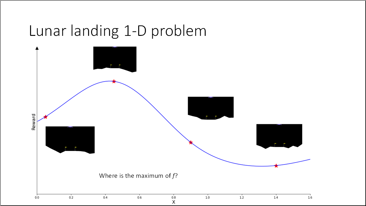
Bayesian Optimization (BO) is one of the most effective and widely used methods for optimizing black-box functions that are unknown and expensive to evaluate. It was originally proposed by the Lithuanian scientists Jonas Mockus, Vytautas Tiešis, and Antanas Žilinskas in 1978. The core concept is to define a prior distribution over the functions and use a decision function to optimally identify the next promising evaluation point. This method was presented by J. Mockus, V. Tiešis, and A. Žilinskas in the paper titled “The application of Bayesian methods for seeking the extremum”.

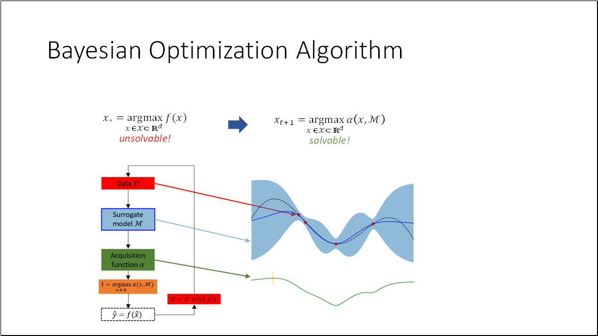
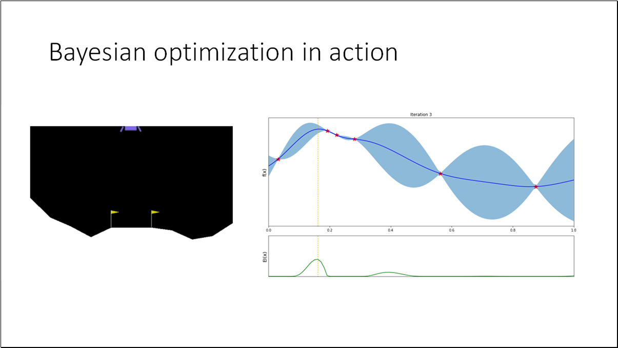
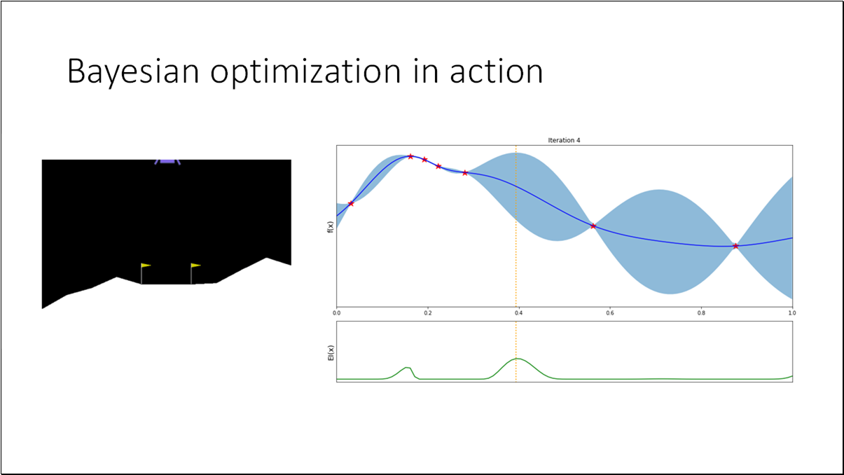
Since we cannot optimize the objective function directly, we utilize a surrogate model as a stand-in. This model aims to closely approximate the objective function while being cost-effective to evaluate. The primary goal of Bayesian Optimization (BO) is to fit the surrogate based on the available data. An acquisition function is then employed to optimize this surrogate model, guiding us to the next most promising point.

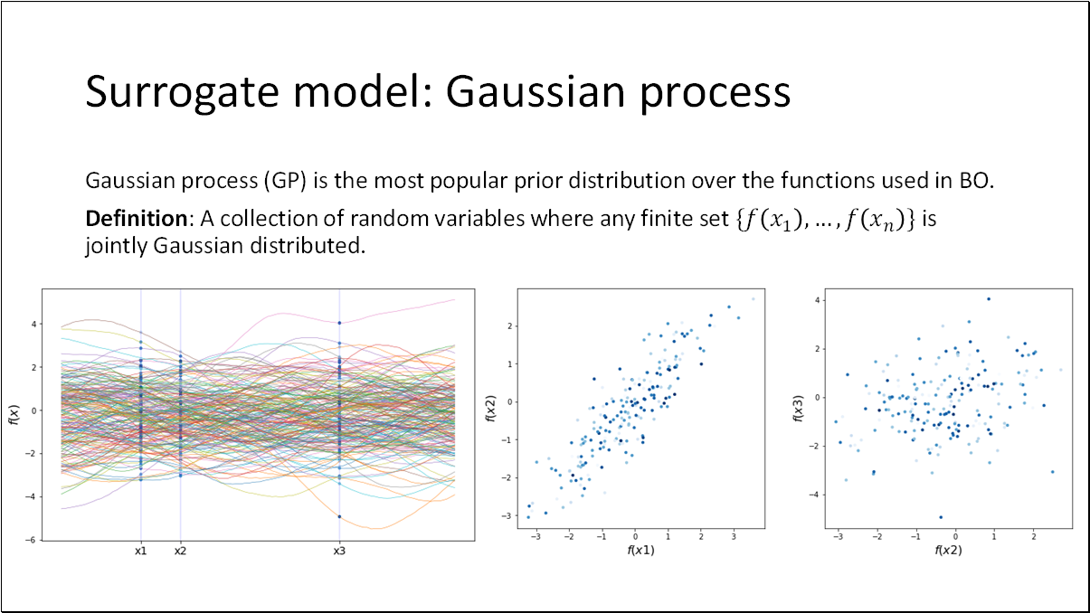
Gaussian Processes (GP) are the most popular prior distributions over functions used in Bayesian Optimization (BO). They are defined as a collection of random variables where any finite set is jointly Gaussian distributed. In simpler terms, if we have random functions and take slices at various locations, plotting the distribution of these values will reveal that they are Gaussian distributed.

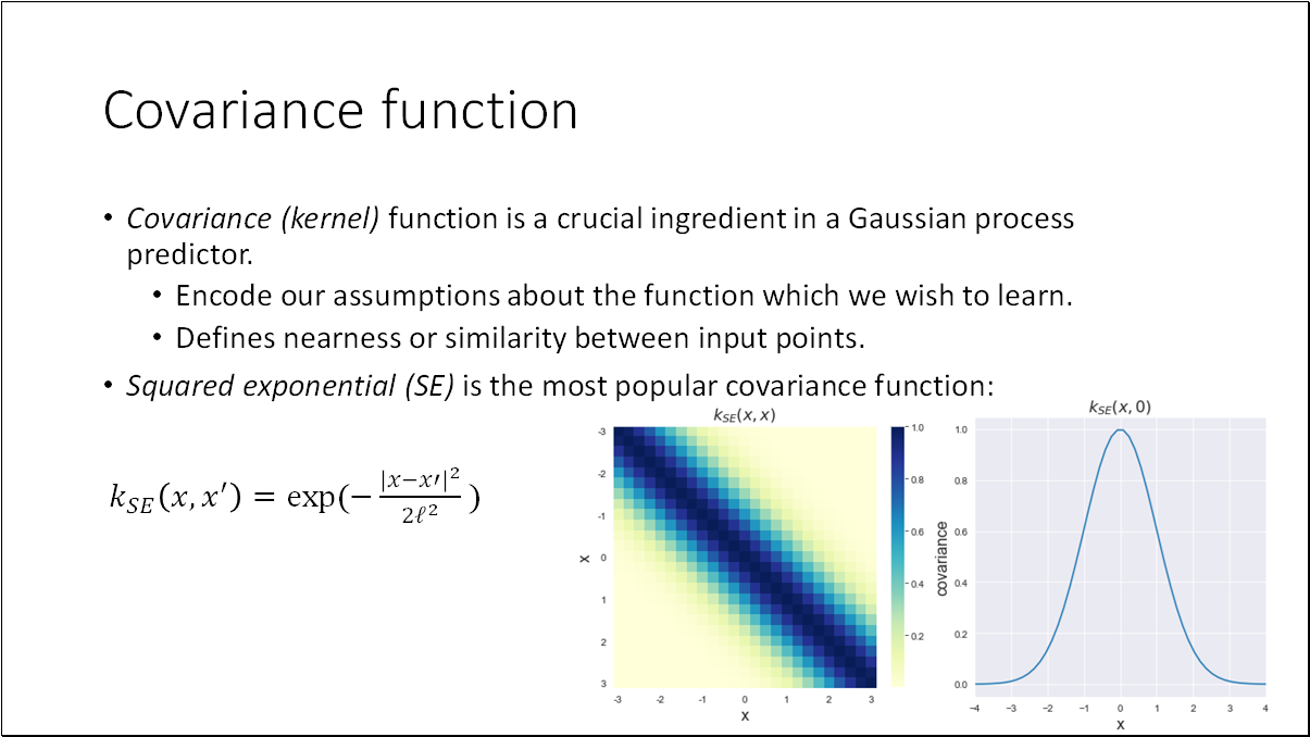
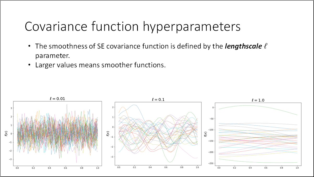
The properties of a Gaussian Process (GP) are primarily derived from the covariance function ( k ). This function encodes our assumptions about characteristics of the function, such as its smoothness, differentiability, and variance. It also defines the similarity between data points. The smoothness of the Squared Exponential (SE) covariance function is determined by the lengthscale parameter; larger values indicate smoother functions.

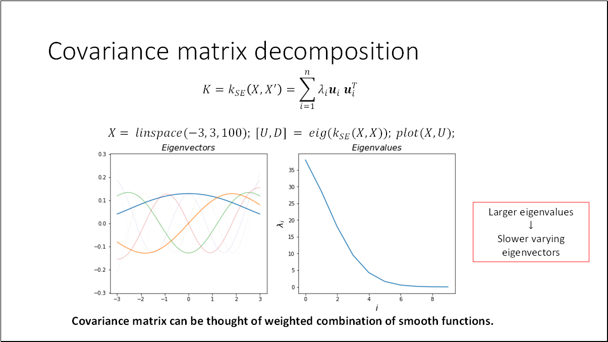
The covariance matrix $K$ can be decomposed using eigenvector and eigenvalue decomposition. I've visualized the ten eigenvectors corresponding to the ten largest eigenvalues. It's evident from the plots that the eigenvectors closely resemble smooth functions. Essentially, the covariance matrix can be interpreted as a weighted combination of these smooth functions. Typically, larger eigenvalues correspond to more slowly varying eigenvectors (e.g., those with fewer zero-crossings). Consequently, high-frequency components in $y$ tend to be smoothed out in practice.

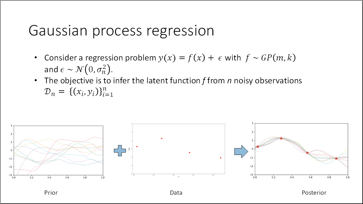
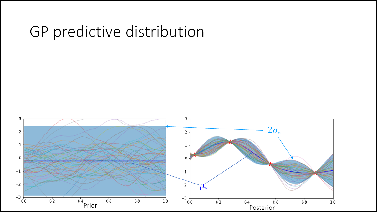
We can consider GP as a regression problem and the objective is to infer the latent function $f$ from $n$ noisy observations.

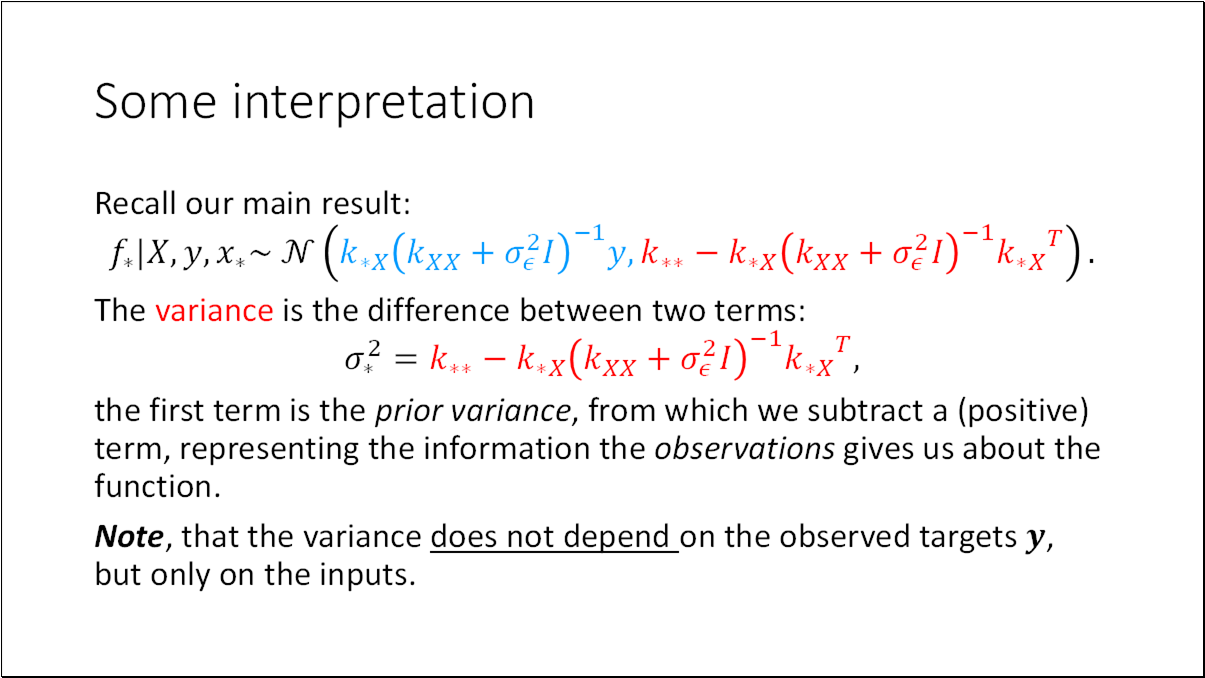
The combination of the prior and the data gives rise to the posterior distribution over functions. The posterior assimilates information from both the prior and the data via the likelihood. To derive the posterior distribution over functions, we must constrain this joint prior distribution to only encompass those functions consistent with the observed data.

The principal notion behind $\sigma_n$ is that when a new observation is added, we recalibrate the noise for all samples. These samples still originate from the same distribution, but when we introduce a new observation $n+1$, our modeled noise deviates from the preceding sample size of $n$ data points.

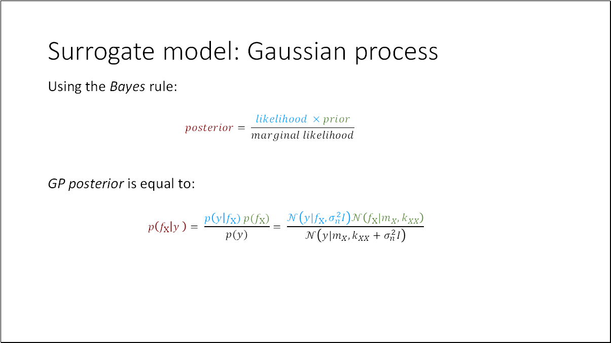
To determine the posterior distribution, we can employ Bayes' rule. This principle states that the posterior is the product of the likelihood and the prior, normalized by the marginal likelihood.

• GP Prior: $p(f)$
• Gaussian Likelihood: $p(y|f)$
• GP Posterior: $p(f|y)$

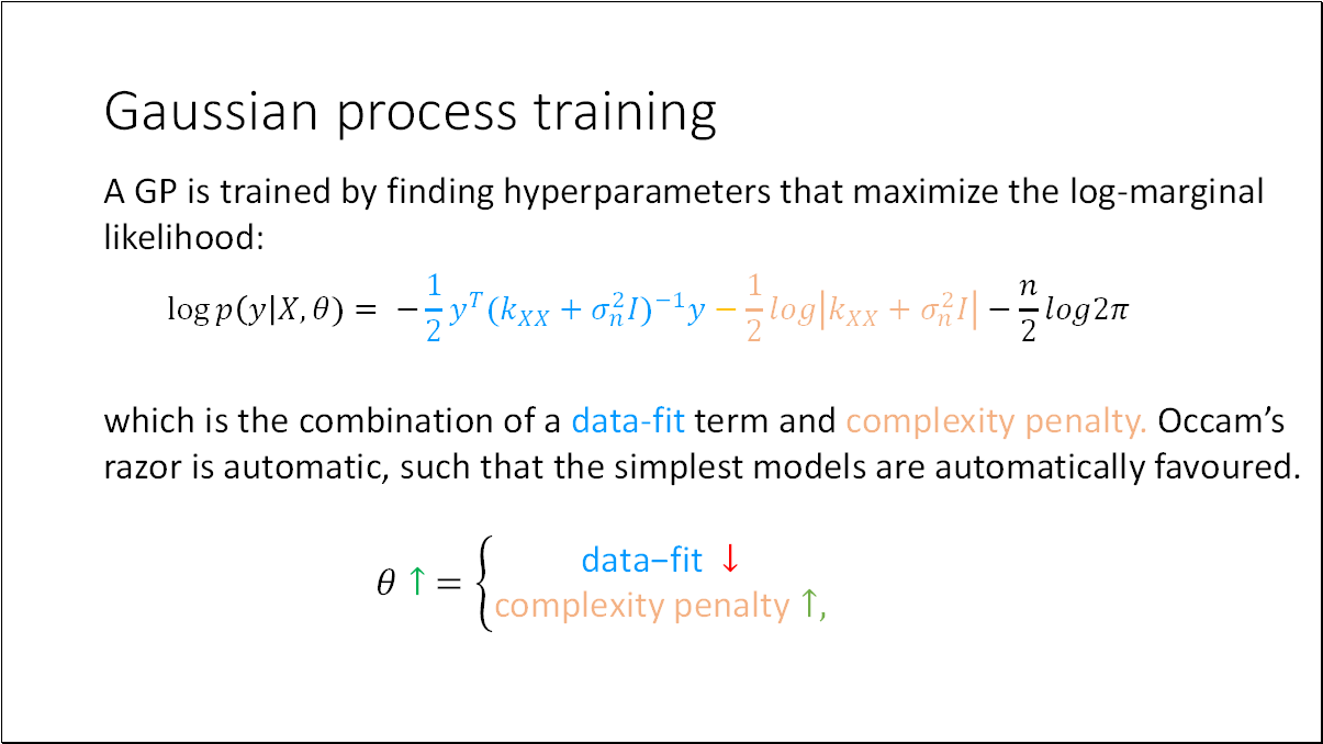
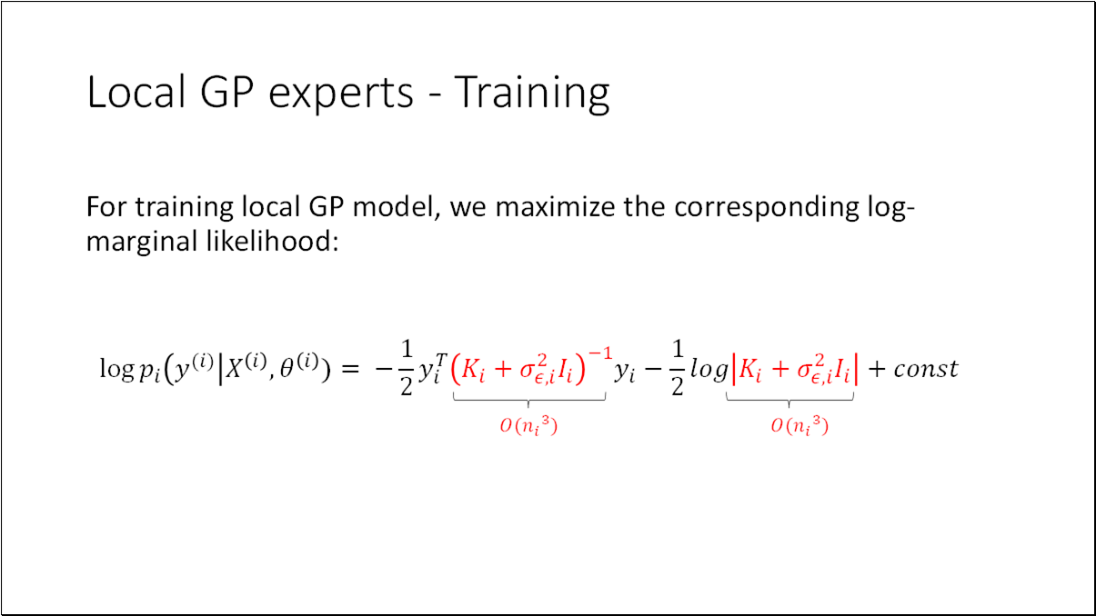
We train GP by finding its hyperparameters that maximize the log-marginal likelihood, such that the simplest models which explain the data are automatically favoured.

Rasmussen, p. 131

The data-fit decreases monotonically with the length-scale, since the model becomes less and less flexible. The negative complexity penalty increases with the length-scale, because the model gets less complex with growing length-scale.

Occam’s razor suggests that in machine learning, we should prefer simpler models with fewer coefficients over complex models like ensembles. Source

The automatic complexity penalty, called the Occam’s factor [^3^], is a log determinant of a kernel (covariance) matrix, related to the volume of solutions that can be expressed by the Gaussian process.

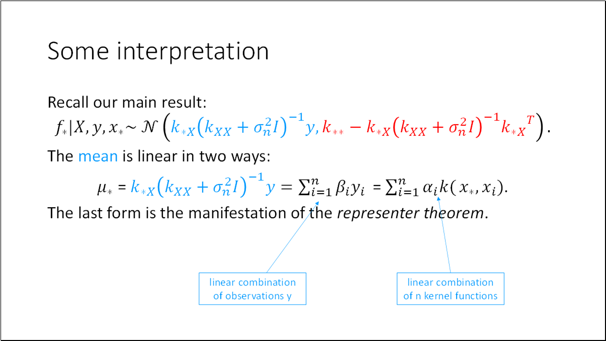
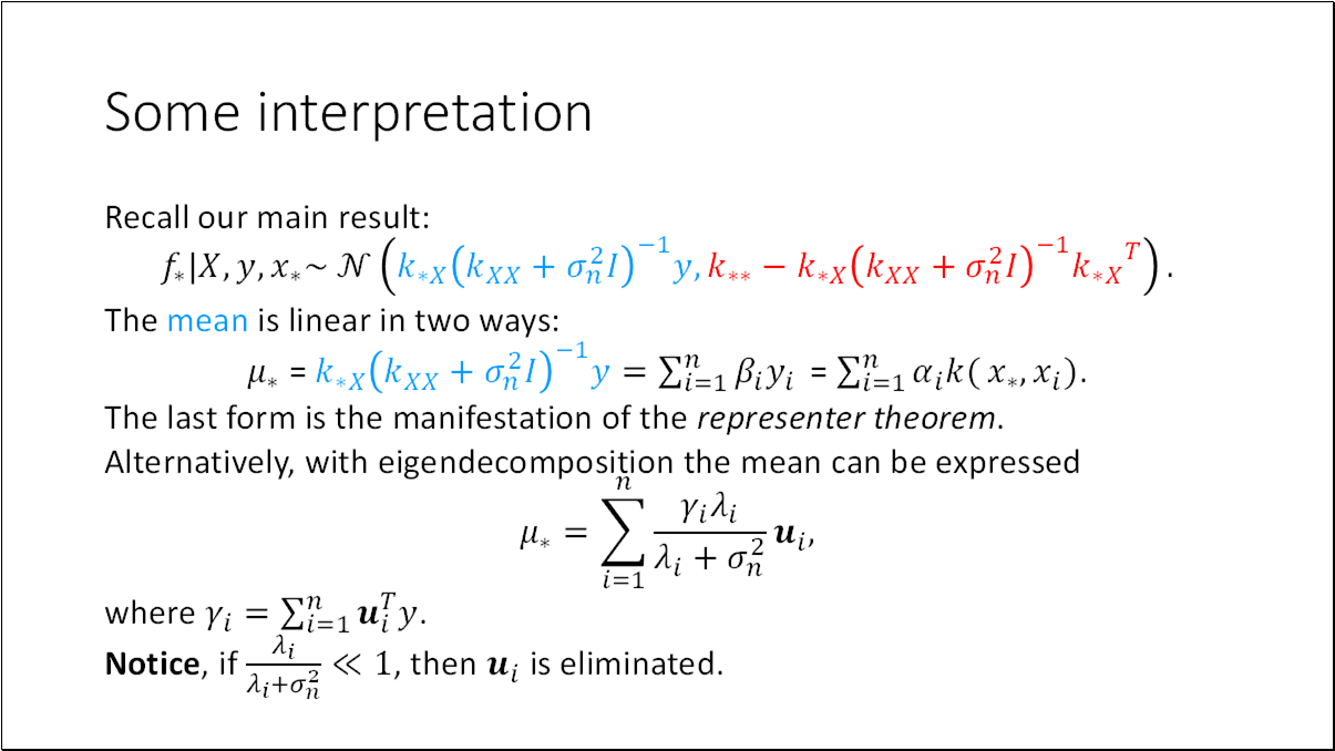
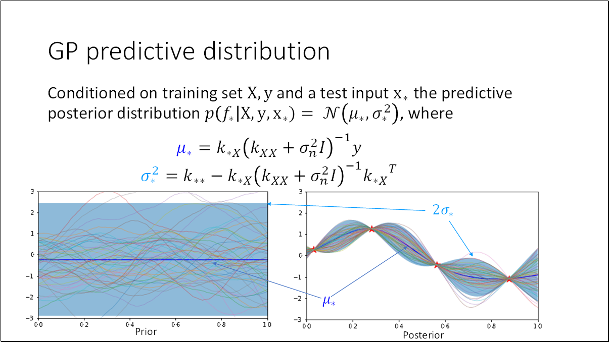
Note first that the mean prediction is a linear combination of observations $y$; this is sometimes referred to as a linear predictor. Another way to look at this equation is to see it as a linear combination of $n$ kernel functions, each one centered on a training point.

The significance of the Representer Theorem is that although we might be trying to solve an optimization problem in an infinite-dimensional space, containing linear combinations of kernels centered on arbitrary points of $x$, it states that the solution lies in the span of $m$ particular kernels — those centered on the training points.

Notice that if $\frac{i}{i + 2n}$ approaches 1 then the component in $y$ along $u_i$ is effectively eliminated. For most covariance functions that are used in practice, the eigenvalues are larger for more slowly varying eigenvectors (e.g., fewer zero-crossings), so that this means that high-frequency components in $y$ are smoothed out.

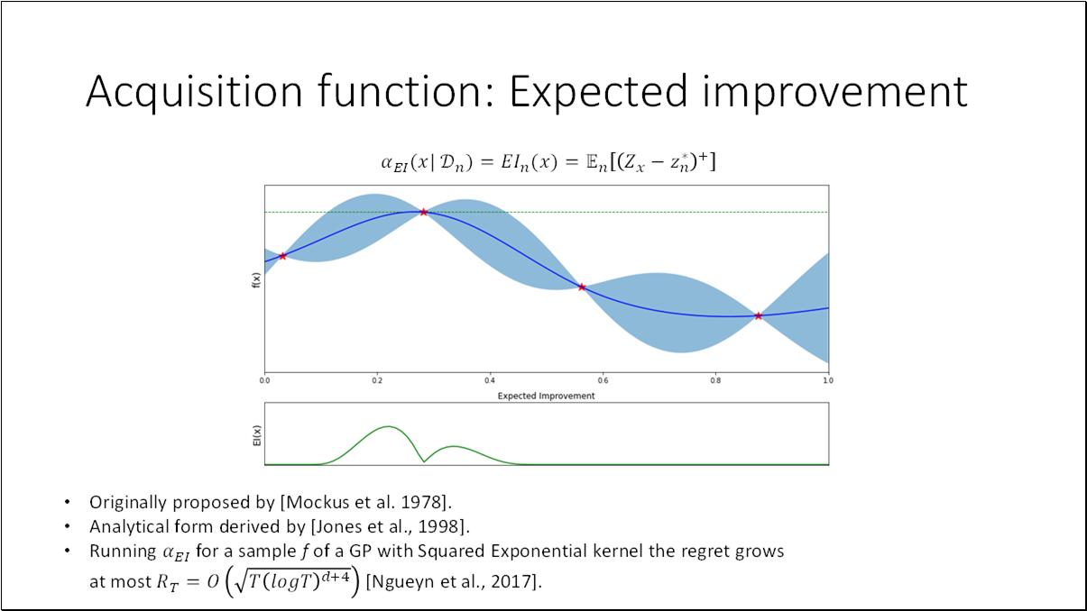
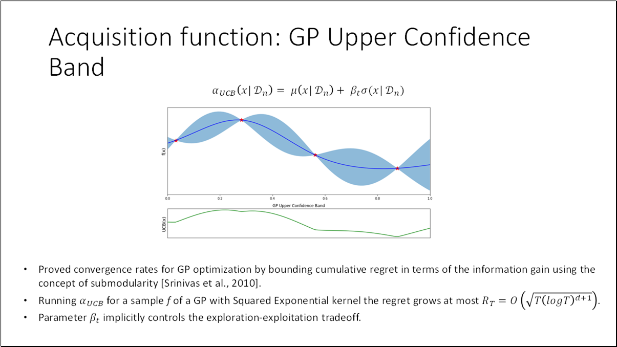
Acquisition function the heuristic used to evaluate the usefulness of one of more design points and deciding where to sample next for achieving the objective of maximizing the black box function.

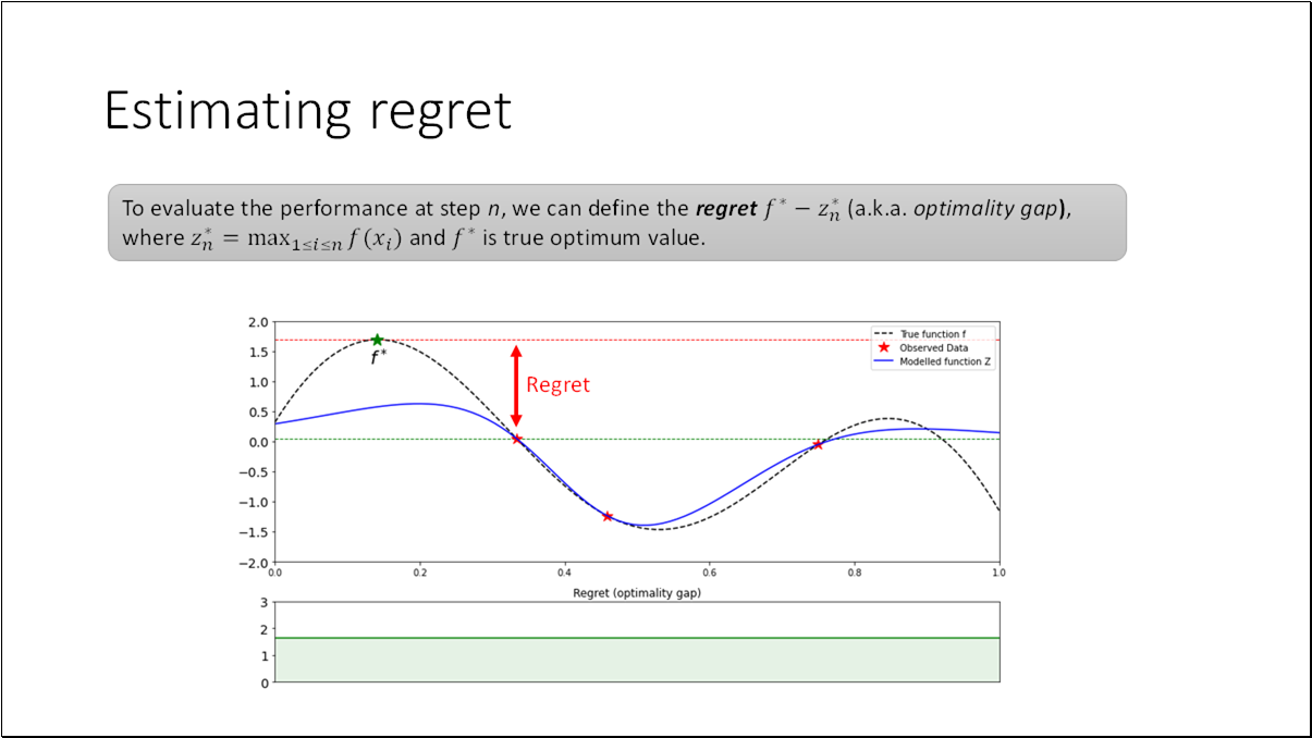
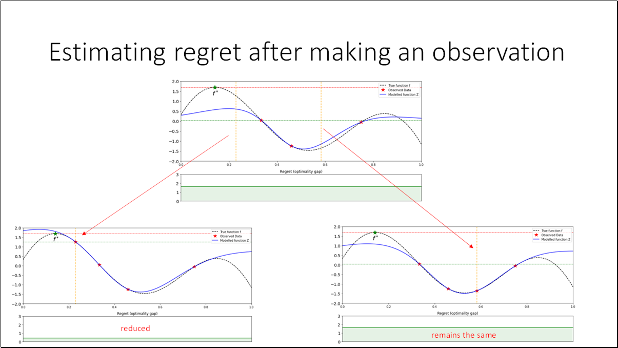
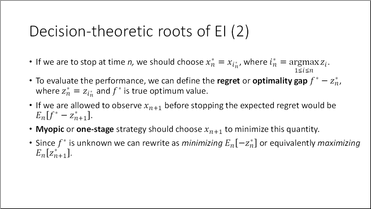
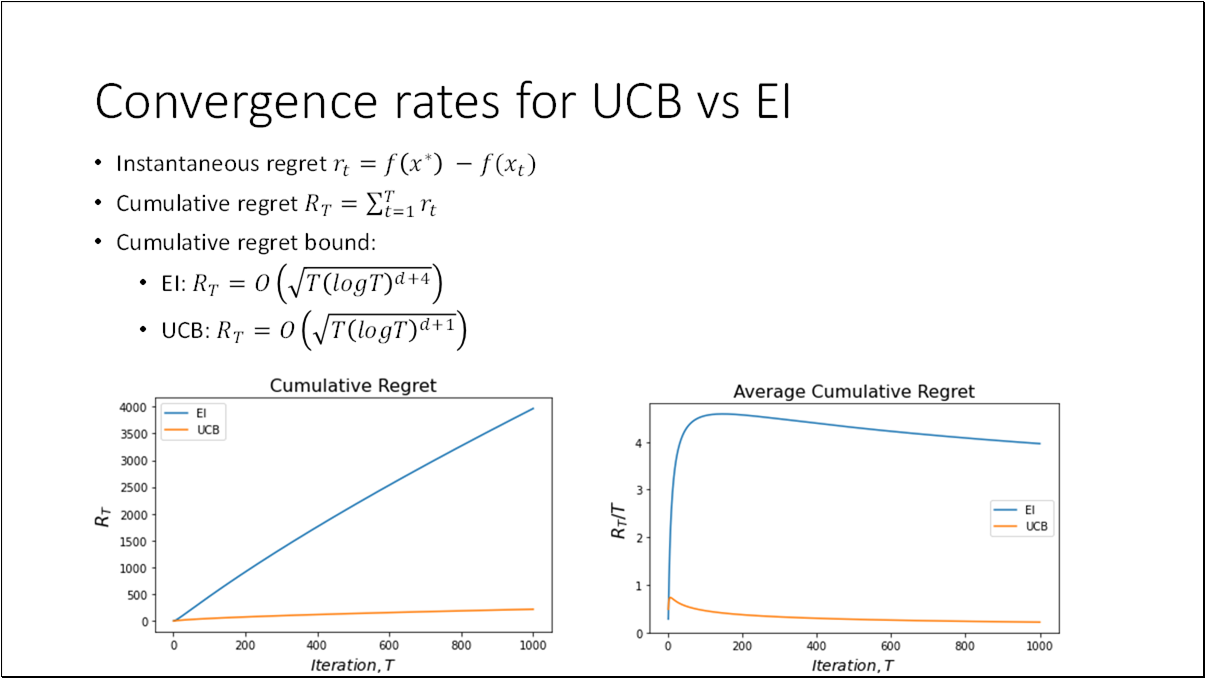
To evaluate the performance at step $n$, we can define the regret $f^* - z_n^*$ (a.k.a. optimality gap), where $z_n^* = \max_{1 \leq i \leq n} f(x_i)$ and $f^*$ is the true optimum value.

• BO is an effective method for black-box functions optimization.
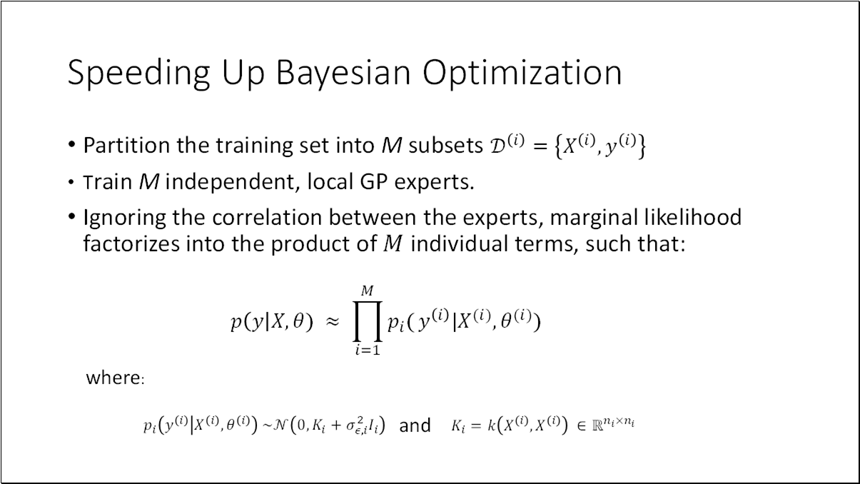
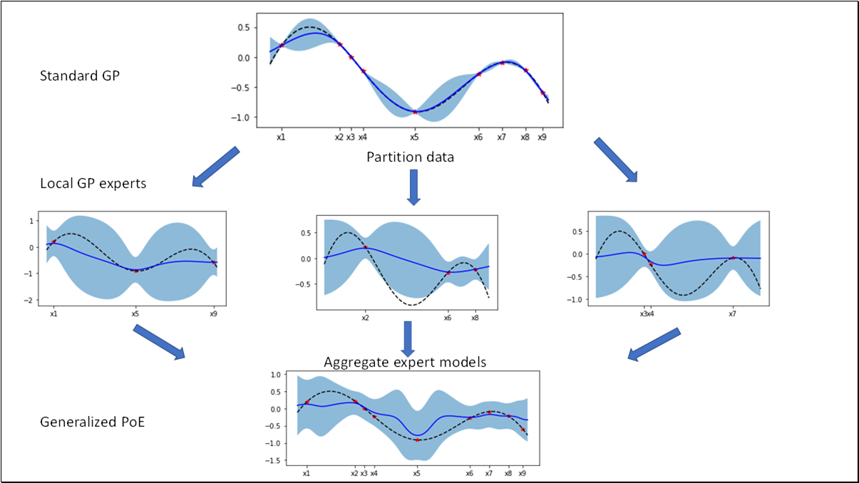
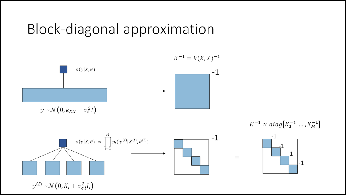
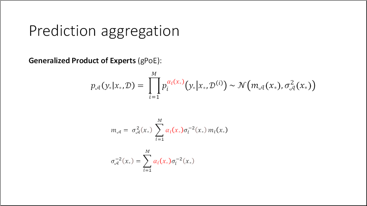
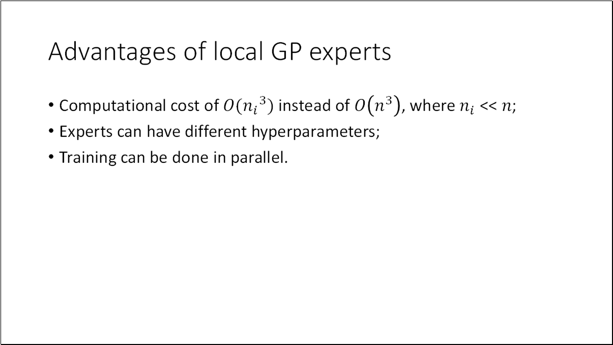
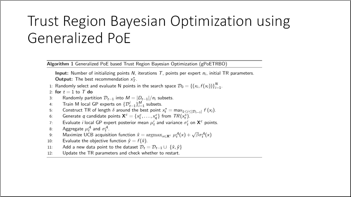
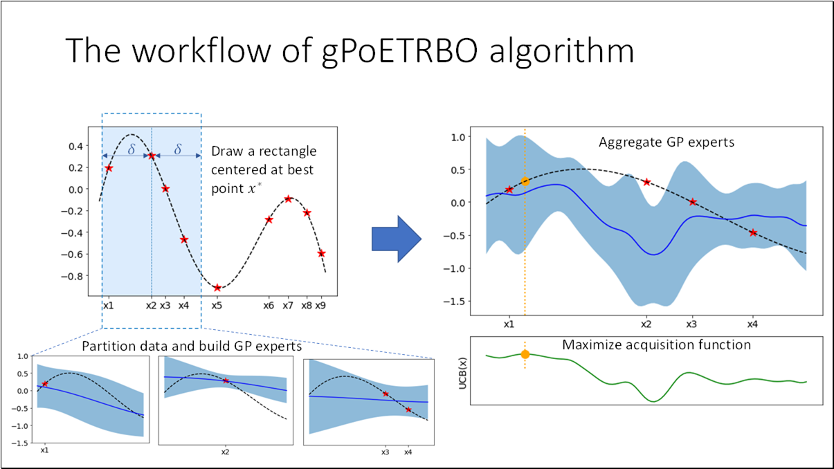
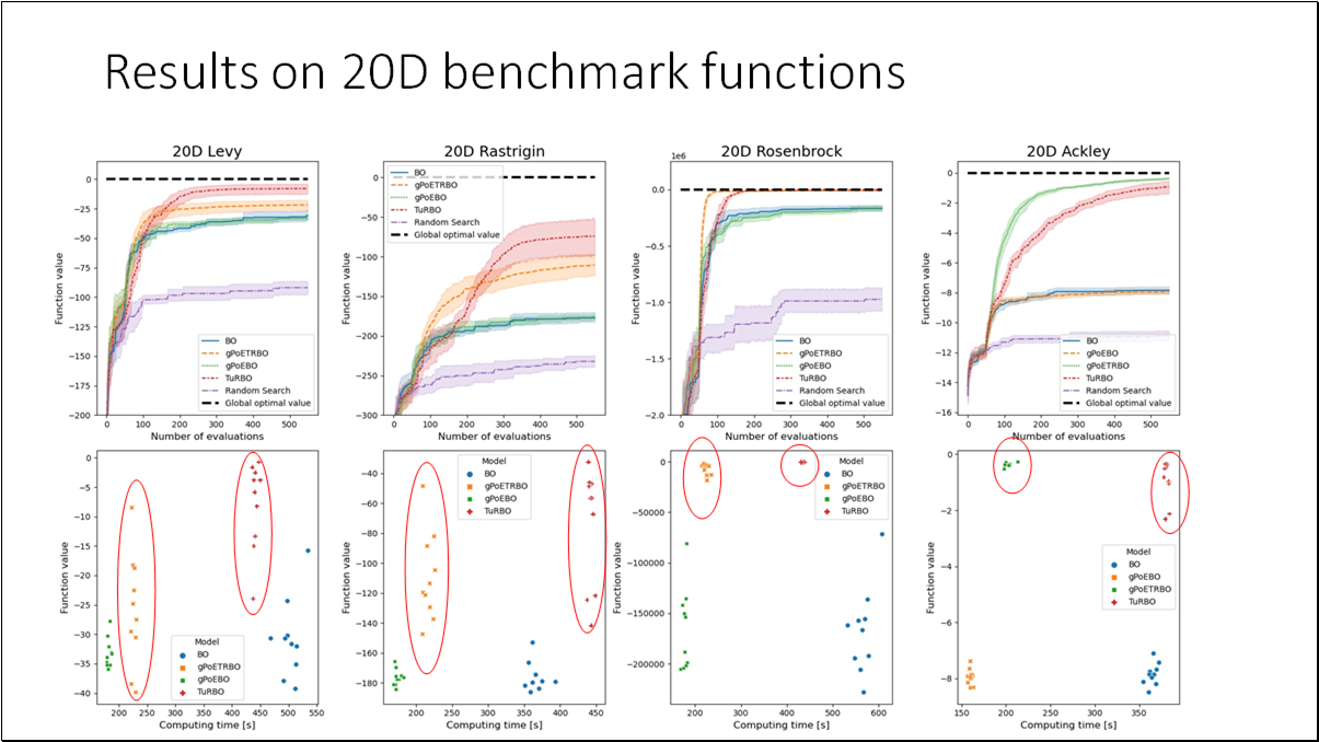
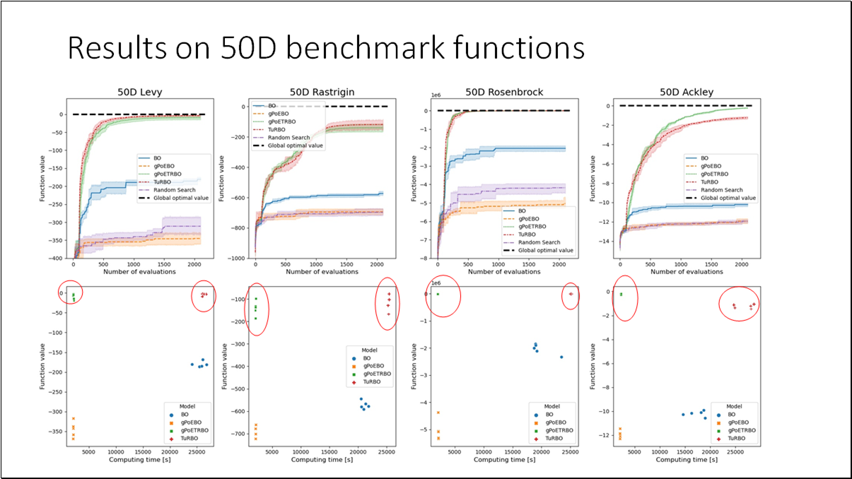
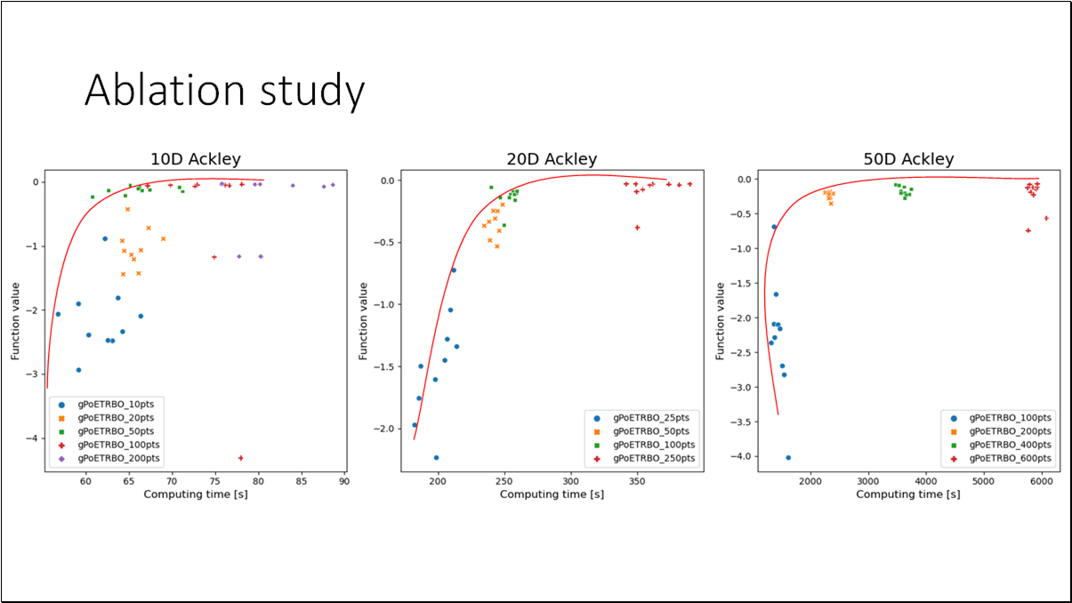
• Generalized Product of Experts model is efficient and scalable replacement for standard GP model used in BO.
• Using this model, we can significantly speed up BO without a loss in accuracy.